
![]()
The program performs inversion of amplitudes of longitudinal (P) and transversal (S) seismic waves as 3-component vectors into the mechanism of the seismic source in the description of shear-tensile crack (STC).
![]()
REFERENCES Document Repository
CATEGORY Source Parameter Estimation
KEYWORDS Seismic event mechanism, Crack source model, Shear-slip and crack opening/closing, Inversion of P an/or S amplitudes, Grid search
CITATION Please acknowledge use of this application in your work:
IS-EPOS. (2019). Mechanism: Shear-Tensile crack [Web application]. Retrieved from https://tcs.ah-epos.eu/
Introduction
The 'Mechanism: Shear-Tensile Crack' application inverts amplitudes of P and/or S seismic phases complemented with the polarity signs, i.e. the particle motion vectors, into the mechanism in the Shear-Tensile Crack description (see, e.g., Šílený, J., 2018. Constrained moment tensors: source models and case studies. In: Moment Tensor Solutions – A Useful Tool for Seismotectonics, Ed. Sebastiano D'Amico, Springer Natural Hazard Series, Springer, ISBN 978-3-319-77358-2 , 213-231). In the current implementation, it is joined with the application reading a seed file and picking the amplitude. If the seismograms processed represent velocity records, we need to pick the amplitude at each station in the peak-to-peak manner, i.e. from first peak of the phase to the second one, see Figure 1.
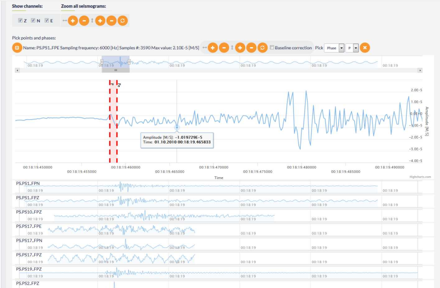
Figure 1. Example of picking of the amplitude of the P-wave from a velocity record.
The more data available, the more is the inverse task constrained. Therefore, it is reasonable to pick amplitudes from all the components of 3-component records. If however some of the components are not of sufficient quality, it is possible to skip them.
The Shear-Tensile Crack source model is described by fou r angles – slope, dip, strike and rake, and a magnitude. The application seeks for the parameters of the model by grid search in two steps: (i) a coarse grid usually across the whole model space, i.e. in the intervals representing the entire definition ranges of individual angles, and (ii) in a fine grid in the vicinity of the best solution found in (i). Definition ranges of the angles are the following:
- slope <-900, +900>
- dip <00, +900>
- strike <00, +3600>
- rake <-1800, +1800>
The value of the step during the coarse grid search is specified in the corresponding box of the input table, see Figure 2.
The fine grid (ii) is specified by defining two integers through the "Advanced options": the first one defines the size of the fine gridding area in multiples of the coarse grid step (in the current example the fine grid interval is <best slope – 50, best slope + 50>, and similarly for the other angles), the second integer defines dividing the course grid step to obtain the fine grid step, here it is one tenth of the coarse grid, i.e. 0.50.
Gridding of the magnitude of the mechanism – described usually as the moment – is different. Obviously, there is no definition range of this parameter. Therefore, for the sake of keeping the evaluation reasonably fast, we take advantage of using an estimate of the source moment obtained from an prior processing. Advantageously, it can be the norm of the moment tensor obtained by inverting the amplitudes in terms of the moment tensor source model first, e.g., by using the application Mechanism: Full Moment Tensor. Then, the value of the moment norm estimate M0 is put in the first box of the input table, see Fig.2. The application defines the interval for gridding of the moment <M0/10, M0*10> and proceeds here on the logarithmic scale with the step 0.1.
Each source mechanism inversion needs the knowledge of the response of the medium, the Green's function. It is a characteristics of the material of the zone depending, in addition, of the configuration of the source and the recording stations. Positions of the stations are obtained from the seed file of the records, coordinates of the source – the hypocenter – must be filled into the table: the latitude, longitude and the depth (Fig.2). For complex structures the evaluation of the Green's function may be difficult. For the sake of simplicity, here we apply the simplest model of the rock mass, namely an isotropic homogeneous medium described by the P and S wave velocities and its density. Regardless its triviality, it may be a good approximation for local underground configurations. The corresponding values of the velocities and the density should be put into the input table (Fig.2). The scaling factor serves for an optional modification of the orders of the Green's function throughout the inversion, the value 1 means no modification of the evaluated Green's function entering the inversion.
Step by Step
After the User adds the Application into his/her personal workspace, the window as shown in Figure 2 appears. The following files are necessary:
- MiniSEED Waveform
- Network inventory
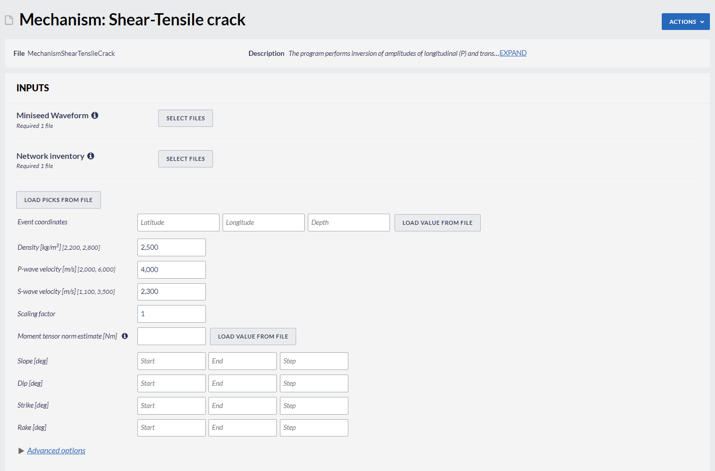
Figure 2. Input window of the "Mechanism: Shear-Tensile Crack" application.
For more thorough instructions regarding uploading necessary files, loading picks from file and picking see FOCI user guide.
The outputs of the application are presented in three sets:
(1) The output values of the parameters of the STC mechanism: slope angle, dip, strike and rake, together with the normalized root mean square value describing the success of the inversion (the value 0 means the perfect fit of the synthetic amplitudes to the data, value 1 no fit). In addition, the output values of the moment tensor corresponding to the resolved STC mechanism are presented, Figure 3.
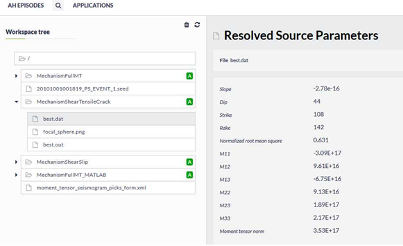
Figure 3. Resolved values of the STC angles slope, dip, strike and rake, normalized root mean square, and components of the moment tensor equivalent to the STC.
(2) The plot of the mechanism in the traditional form of the display of zones of compression of the P-waves generated by the resolved mechanism (generalized "beach ball"), Figure 4.
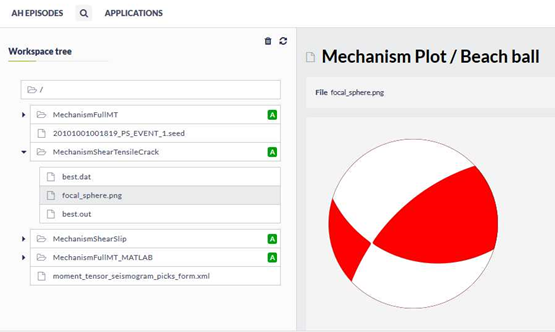
Fig.4 Plot of the mechanism in the generalized form of the traditional "beach ball".
(3) The decomposition of the moment tensor corresponding to the resolved STC mechanism into the volumetric (isotropic) component (V), the double-couple component (DC), and the compensated linear-vector dipole (CLVD). In addition, two equivalent sets of the dip, strike and rake angles corresponding to the resolved DC are presented, Figure 5.
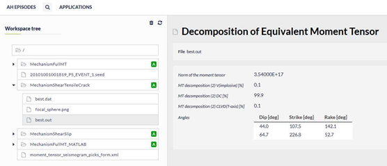
Figure 5. Norm and decomposition of the moment tensor, equivalent to the resolved STC.

Overview
Content Tools
![]()
EPISODES Platform is maintained by the TCS AH Consortium![]() . © 2023 IG PAS & ACC Cyfronet AGH
. © 2023 IG PAS & ACC Cyfronet AGH