Page History

Some visualizations connected with the Applications are described in this section. There are some special visualizations for mining-induced seismicity. They can be accessed from the 'Mining Front Advance' file (Figure 1), uploaded to the workspace from the AH-Episode database.The User may click on 'Actions' tab, then on 'USE IN VISUALIZATION' tab, and then select among the two visualizations shown in the right red panel of Figure 1 (for additional visualization - 'Integrated episode data visualization', see "AH-EPISODES Chapter").

Figure 1.

•  Seismic Activity with Front Advance: This is an application dedicated to mining induced Episodes and is directly connected with the 'Time Dependent Seismic Hazard' Application. Figure 1b shows the input that is necessary to perform this visualization:
  1. Input files are 'Mining Front Advance' and the corresponding seismic catalog, imported from the AH-Episode database.
  2. Chose line date: The User selects the date that the front is in a certain position, either by selecting a date from the available list, or by clicking on a certain line in the 'Front Advance Plot' (right part of Figure 1b.)
  3. Select Magnitude Column: The user may click on the small arrow in the respective tab in order to chose among different magnitude scales, in the cases where they are available (e.g. ML, Mw, etc).
  4. Mmin: The User now is requested to chose the minimum magnitude (completeness level of the catalog). This can be done in two ways. The first is to type a single magnitude value in the empty box, possibly after he/she has performed an individual analysis (see application 'Magnitude Completness Estimation' - MCE)    %In my opinion it is worth to explain all acronyms beforehand%. The second is to graphically select the minimum magnitude from the Normal or the Cumulative histograms, which are available after clicking on the respective tabs. In both cases there is option to alter the step of the histogram's bars and to select between linear and logarithmic scale of the Y-axis for the plotting. The magnitude range is also shown in the screen.  
  5. Margin along front strike: The distance (margin) along the front strike is requested in this field. This distance is equal for both directions of the front strike. Events will be spatially constrained by this margin together with the 'Distance along the front advance' (see field below).
  6. Distance along the front advance: The distance along the front advance is requested in this field. This distance is equal for both sides of the front (i.e. in front of and behind the front). Events will be spatially constrained by this margin together with the 'Margin along the front strike' (see field above).
  Once all the parameters are set, the User may click on the 'RUN' button (green button, at the bottom of figure 1b), to initiate the visualization process

Figure 1b.

The result is a map similar to the one demonstrated in Figure 1c.

Figure 1c.

Four vectors with output results, corresponding to data extracted are also produced and they are the front position, the latitudes, longitudes and magnitudes of the events. These vectors are available for further processing and can be used as input for other applications. By clicking on any of them in the list, the values of the vector appear on the screen.

•  Front Advance Histograms Visualizations: This is also an application dedicated to mining induced Episodes and is directly connected with the 'Time Dependent Seismic Hazard' Application. It provides histograms of seismic events and seismic energy release for constant steps of mining front advance. The data needed for this application comes from the '"AH Episodes" (see this chapter) and in particular 'Bobrek Mine seismic catalog' and 'Bobrek mine front advance', as depicted in Figure 2, next to "Using Seismic catalog" and "Using mining front advance", respectively. Any other, previously filtered catalog can be introduced as well. In addition, the front window size is requested to be set by the user (in meters).

Figure 2.

The results will be demonstrated after clicking on the 'Run' button (green box in Figure 2). An example of the resulting histograms is shown in Figure 3 ('events histogram' - above, 'energy histogram' - below). Zooming in/out and interval/cumulative histogram plotting are available for both events and energy charts. Options for linear/logarithmic scale of the x-axis and y-axis are available only for 'energy histogram'. The results are also available in numerical format.

Figure 3.

•  Integrated episode data Visualization: This is an alternative way to access integrated Episode data visualization, already described in "AH Episode Chapter".

...

•  Waveform Viewer Guide: Waveform viewer is a seismic waveform processing tool. The User may observe, interact and elaborate waveforms corresponding to signals recorded by seismic stations and perform various actions such as phase determination and point picking. These pickings are saved by the system and can be further used in waveform-based applications such as 'Spectral Analysis', 'Source Localization' and 'Moment Tensor Inversion'. The options provided by the 'waveform viewer' are described in Figure 74:
  When clicking on one waveform, additional options appear. The user selects the component(s) that he/she wishes to be displayed on the screen. East-West, North-South, Vertical.

Figure 74.

1. The user selects the component(s) that he/she wishes to be displayed in the screen. East-West, North-South, Vertical.
2. Horizontal zooming in-out.
3. Vertical zooming in-out.
4. Undo all zooming.
5. Select between phase (start and end point) picking and single point picking.
6. Only P-wave is enabled in this Application (In other Applications, selection between P-wave and S-wave picking are possible, see "Waveform viewer guide" in "Visualization" chapter).
7. Undo picking.
8. Horizontal zooming tool. The User may alternatively zoom in-out the waveform by clicking on this small vertical bar and move the mouse left-right. The User may also click and drag the selected (shaded) part of the waveform left and right.
9. Collapse the details of the waveform.
10. Move the selected (zoomed) part of the waveform left-right.

...

The User has to pick a starting and an ending point from the Vertical component of a station (**Z channel - see Figure 85). Then, he/she has to repeat this picking for the other stations.

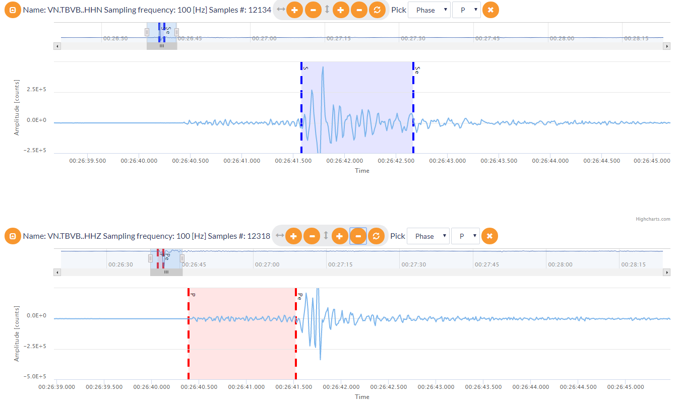
Figure 85.

The number of the seismograms and P-wave phases picked, are updated, each time the User selects makes a new picking.

...

• 1-D and 2-D plots - including 1-D and 2-D plots with secondary Y-axis (Figure 96): These plots give the capability of choosing between linear and logarithmic scales for X and Y axes (ticking on small boxes, Field 1, Figure 96) and selection of diverse graphic views among scatter plot, spline, column and line. Plotted parameters may be hidden and re-appear by clicking at the legend (Field 2, Figure 96). By holding the cursor still onto an option or in a figure element [e.g. bar in histograms or points in scatter plots], information on this option or element appears on the screen (Field 3, Figure 96). Many figures have enabled zooming services for focusing in a specified range among the values. This is achieved by clicking at a point of the figure and dragging the mouse cursor either leftwards or rightwards. Instructions are shown at the bottom of the figure as well (field 7, Figure 9).Zooming can be reset by clicking on the 'Resert Zoom' tab shown in Field 4 of Figure 96. The user may save a selected figure (Field 5, Figure 96) in one or more of the following formats by clicking on the square panel: .png, .jpeg images, .pdf document or .svg vector image. Alternatively, for some figures the user can download the corresponding data and save them in .csv format in order to use it for further analysis. The figures can also be printed (also from Field 5, Figure 96).

Figure 96.

• In addition to the previous mentioned options. Histograms, Cumulative Histograms and Reverse Cumulative Histograms also provide the possibility for the user to adjust the step (width) of the x-variable (indicated in the red box, Figure 10)7.

Figure 107.

• 3-D images are equipped with a rotation function (instead of zooming), activated by holding the left click and moving the mouse Figure 118. 

Figure 118.

•  Maps Guide: All google basemaps have in effect the following well known tools (an example is demonstrated in Figure 129): Moving at any direction in the map by clicking and dragging the hand pointer throughout the map. The street-view imaging tool can also be applied (Field 1, Figure 129). Zooming in/out can be performed mouse rolling, or, alternatively, by using the zooming tool (plus-minus boxes and small bar) shown in Field 2 of Figure 12Figure 9. The map scale is updated after any zooming action and is shown at the right bottom corner of the map (indicated by the blue frame in Figure 12). The User is also given the chance to select between Map view and Satellite image (Field 3, Figure 129). Terrain and Labels, respectively, can be shown or hidden. Finally full screen mode can be activated after clicking in the "Full Screen" tab (Field 4, Figure 129).  
  

 Figure 129.