Page History
...
- Select Magnitude column:The user may click on the small arrow in the respective tab in order to chose among different magnitude scales, in the cases where they are available (e.g. ML, Mw, etc).
- Mmin range:The User now is requested to chose the minimum magnitude (completeness level of the catalog). This can be done in two ways. The first is to type a single magnitude value in the empty box, possibly after he/she has performed an individual analysis (see MCE service). The second is to graphically select the minimum magnitude from the Normal or the Cumulative histograms, which are available after clicking on the respective tabs. In both cases there is option to alter the step of the histogram's bars and to choose between linear and logarithmic scale of the Y-axis for the plotting.
- Time range: The User may further filter the selected dataset by defining the starting and ending data of the period that he/she wishes to study. A calendar appears on the screen after clicking in the empty boxes next to "Start" and "End" fields. Alternatively, the User may graphically select a time window, after clicking on 'Seismic Activity Plot' tab. A cumulative count of events plotted against time appears and the User can click on certain points of this plot to define the starting and ending time of the time period of interest (Figure 2). Note that this selection is optional. If no dates are entered, the entire dataset remains for the analysis.
- Significance level: The User is requested to enter the significance level, a, for the null hypothesis rejection (0<a<1)
- Distribution: he user may click on the small arrow in the respective tab in order to chose between 'exponential' and 'weibull' distribution
- Monte Carlo Trials: number of Monte Carlo Trials for distribution parameters confidence Intervals evaluation. Should be an integer in the range [100-50,000]
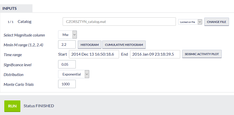
Figure 1. Input window of Inter-event Time Distribution Analysis.
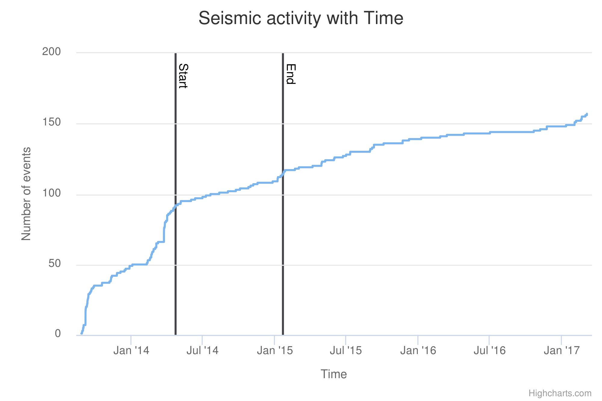
Figure 2 Seismic activity with time plot.
After defining the aforementioned parameters, the user shall click on the "Run" button (Figure 1) and the calculations are performed. The output is soon to be created.
...
- A matlab output file ('stattest_output.mat' - Figure 3) with parameters are displayed on the screen and can be downloaded or used for visualization (click on 'SHOW' tab, Figure 3)
- An ascii report file ('report.txt' - Figure 3) which includes all a summary of input/output data and can be downloaded.
- A plot ('plout_output.mat' Figure 3) of the inter-event time distribution, the best fit curve, and its 2.5 and 97.5 confidence bounds (Figure 4)
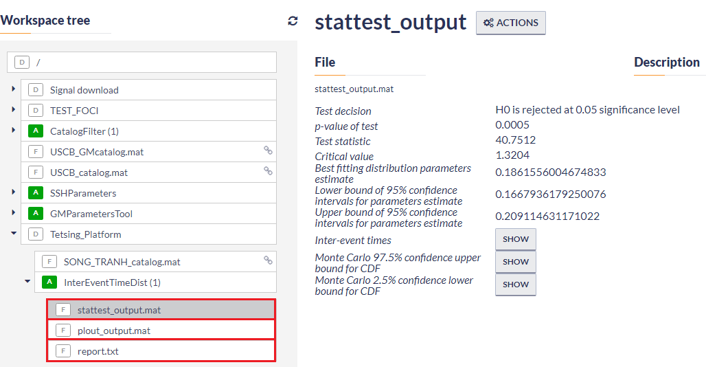
Figure 3. Results of the Inter-event Time. Distribution Analysis.
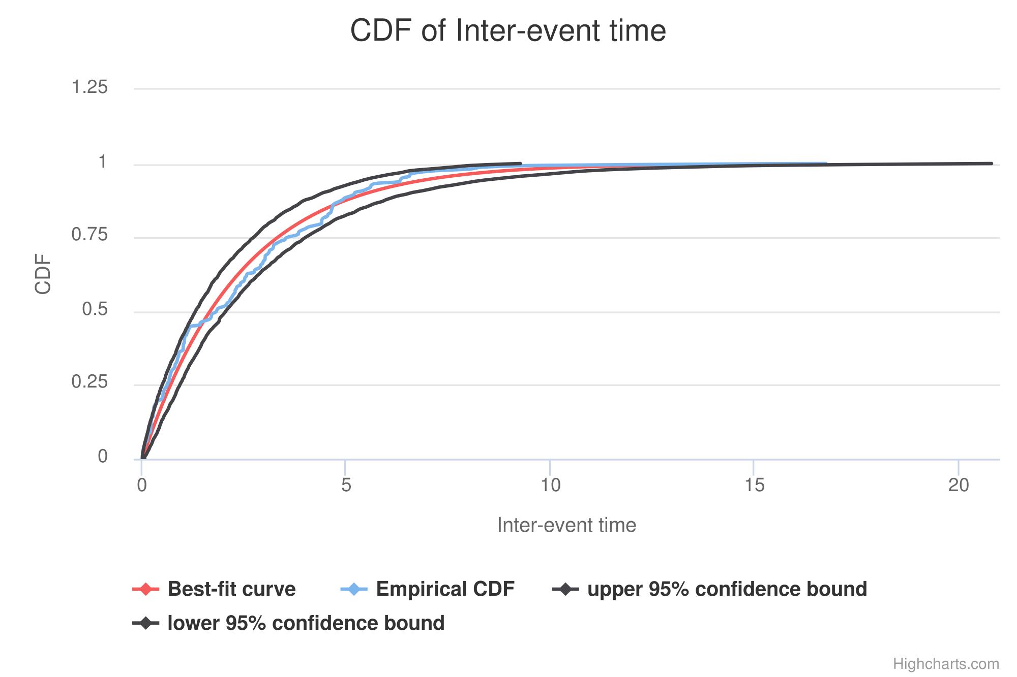
Figure 4. . Cumulative Distribution function of the Inter-event Time.
Overview
Content Tools