Page History
| Anchor | ||||
|---|---|---|---|---|
|
| Info |
|---|
To estimate time-dependent values of seismic hazard parameters: the activity rate, the Gutenberg-Richter b-value, the return period and the exceedance probability for a prescribed area. The parameter values time windows considered for the time moment t are estimated optionally either from events that occurred in dt time units preceding t, where dt is kept constant, or from n last events before t, where n is kept constant. Four magnitude distribution estimation methods are supported: maximum likelihood using the unbounded Gutenberg-Richter relation based model, maximum likelihood using the upper-bounded Gutenberg-Richter relation based model, unbounded non-parametric kernel estimation, upper-bounded non-parametric kernel estimation. The upper limit of magnitude distribution is evaluated using the Kijko-Sellevol generic formula.analysis are graphically selected by the user from production parameter plots. In such way these windows and the derived hazard parameters are directly associated to anthropogenic activity. For the magnitude distribution estimation methods please refer to the “Stationary Hazard” application. |
REFERENCES Document Repository
CATEGORY Source Parameter Estimation, Probabilistic Seismic Hazard Analysis
KEYWORDS Statistical analysis, Probabilistic seismic hazard analysis, Time-dependent hazard, Production-dependent hazard, Production - seismicity interaction
CITATION Please acknowledge use of this application in your work:
IS-EPOS. (2017). Estimation of source parameters in time-varying production parameters geometry [Web application/Source code]. Retrieved from https://tcs.ah-epos.eu/
Step by Step
The input data required for Estimation of source parameters in time-varying production parameters geometry application is a catalog containing seismic events and GDF parameter file (with single time-correlated parameter). The User enters his/her personal workspace and selects a seismic events catalog and a time-corelated parameter, that are already uploaded (see "AH Episodes" chapter).
For using a selected catalog for Estimation of source parameters in time-varying production parameters geometry application, the User shall click on the 'Actions' tab and then select consecutively, 'USE IN APPLICATION' and 'Estimation of source parameters in time-varying production parameters geometry', as highlighted in Figure 1.
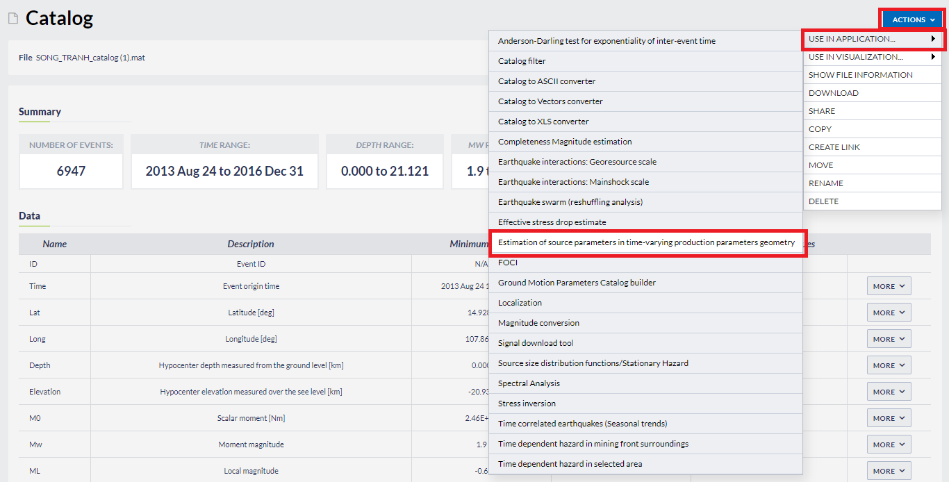
Figure 1. Selection of the application from the data uploaded in the workspace
Once the application has been selected the User is requested to select options and fulfill some fields with parameter values needed for the analysis (see the following Figures). These parameters are:
Catalog: A catalog has been already uploaded since the previous step, however, the User has the chance to select a different dataset, either from another episode or the any dataset after performing some processing/ filtering.
GDF with single time-correlated parameter: The User needs to select, the previously loaded time-correlated production parameter of his/her choice.
Time unit: There are 3 options for this parameter, which are shown after clicking on the small arrow in the box: Day, Month, Year. The time unit will be stored and all the calculations hereinafter will be performed according to this unit.
Mmin: The User now is requested to chose the minimum magnitude (completeness level of the catalog). This can be done in two ways. The first is to type a single magnitude value in the empty box, possibly after he/she has performed an individual analysis (see "Completeness Magnitude Estimation", CME Application). The second is to graphically select the minimum magnitude from the Normal or the Cumulative histograms, which are available after clicking on the respective tabs. In both cases there is option to alter the step of the histogram's bars and to select between linear and logarithmic scale of the Y-axis for the plotting.
Magnitude distribution estimation method: Four different methods are available in the IS-EPOS platformEPISODES Platform: The Unbounded Gutenberg-Richter, the Upper-bounded Gutenberg-Richter, the unbounded non-parametric and the Upper-bounded non parametric estimations. To select one of the aforementioned methods of analysis, the User has to click on the arrow in the respective box.
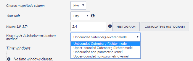
Figure 2. Input parameters selection
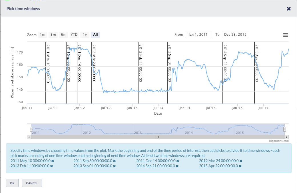
TIme windows: The user need to specify at least two time windows over for the analysis. Time windows can be selected from the plot of the chosen producion parametr, as shown on the figure below:
Magnitude: Magnitude for which the parameters will be calculated.
Period length (for exceedance probability): Duration of time period for which exceedance probability will be estimated for the magnitude specified above.
After selecting all the parameters needed the User may click on the run button  button, for the calculation process to be initiated.
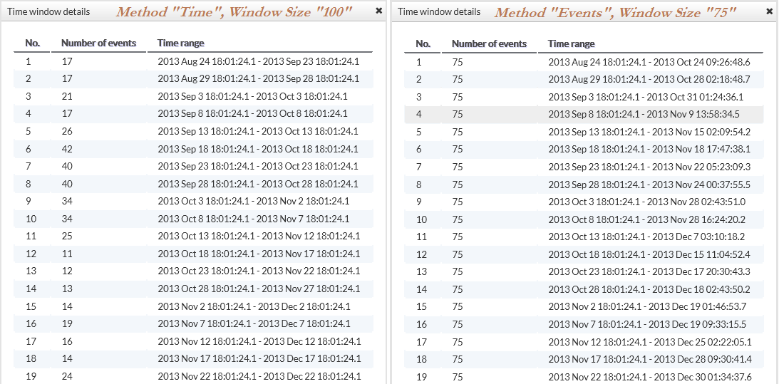
Figure 4. Data windows determination: The time window step is set to 5 days in both cases. Notice that the each starting date has 5 days difference from the previous one. Left frame: Parameters set are 'Time window size' equal to 100 days and 'Method of creating windows' selected to be 'TIME'. In this case the number of events differs in each dataset, but the time range (difference between ending and starting dates) is 100 days for all the datasets. Right frame: Parameters set are 'Time window size' equal to 75 (events) and 'Method of creating windows' selected to be 'EVENTS'. In this case the number of events the same in all dataset and equal to 100, but the time range (difference between ending and starting dates) is different for each dataset.The results of the process include:
- Information on the showing time windows created (Figure 4), shown after clicking on the 'Show details' tab. details:
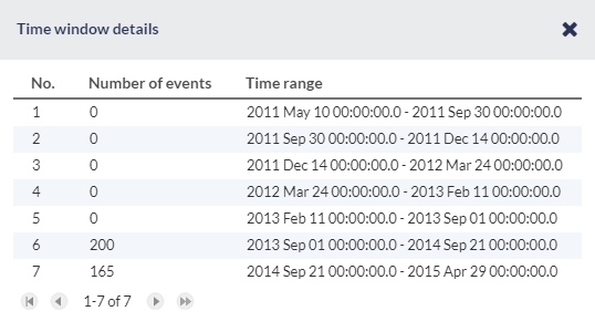
- Numerical parameters resulted by the process, stored in the system, in the current folder (Figure 5). These outputs are available for the User for demonstration and plotting (when available).

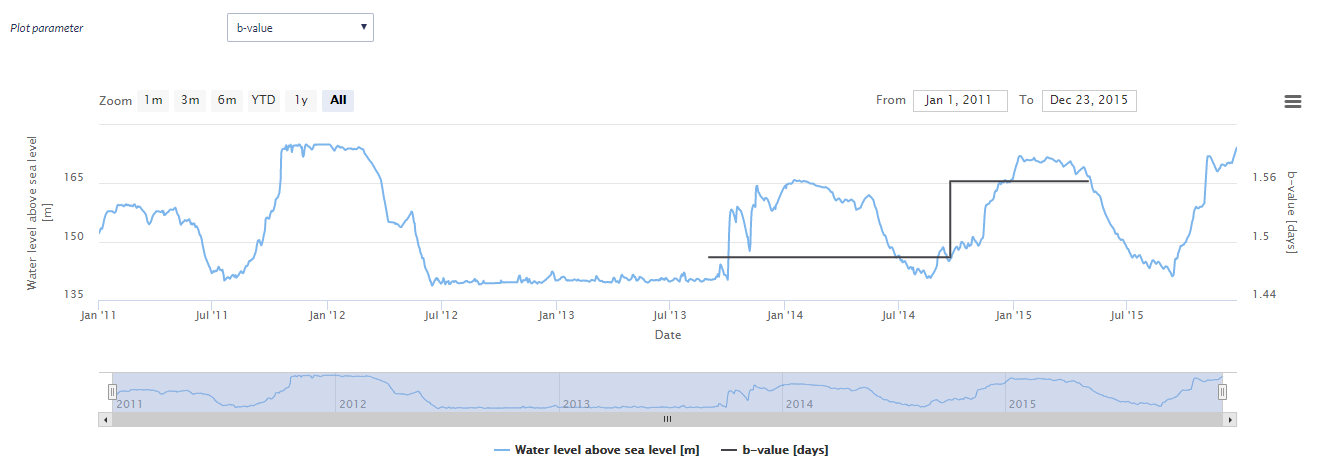
- b-value and mean activity rate (Figure 6)overlaid with plot of the production parameter of the user choice. Note that b-value is not plotted (and not estimated all) if a non-parametric approach is selected as 'Magnitude distribution estimation method'.
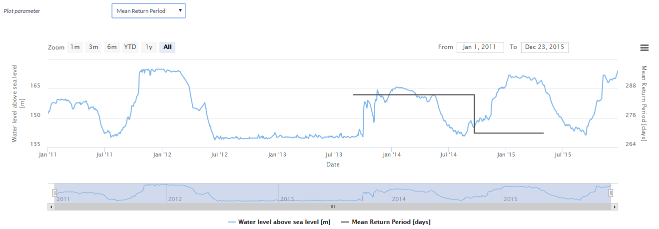
- Mean return period vs time (Figure 7).
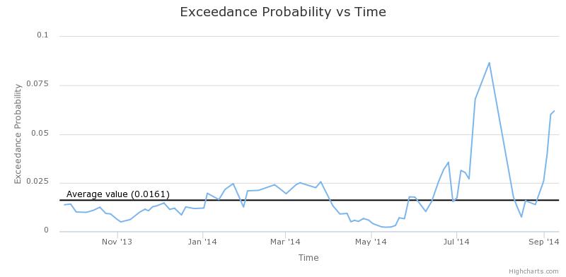
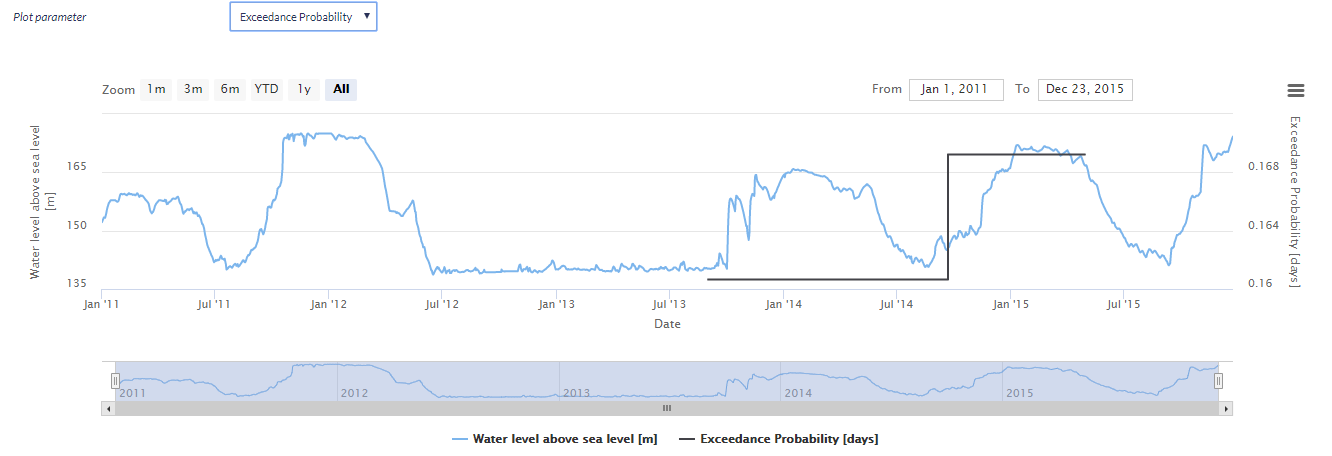
- Exceedance probability vs time (Figure 8).
NOTE that figure have enabled the zoom option, the scatter/line.spline chart type and linear/logarithmic scale of the Y-axis option.
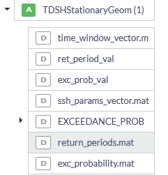
Figure 5. Outputs of the application
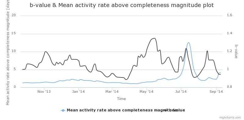
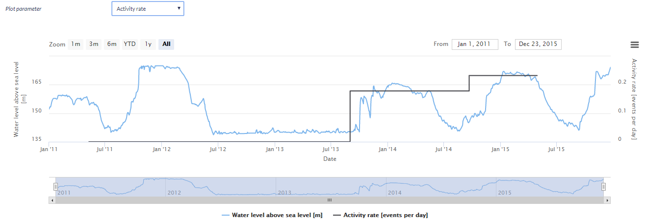
Figure 6. Output graph Mean Activity Rate

Figure 7. Output graph of hazard parameter: Mean Return Period
- Activity rate plot overlaid with plot of the production parameter of the user choice.
- Mean return period plot overlaid with plot of the production parameter of the user choice.
- Exceedance probability plot

Overview
Content Tools