Page History

...

For a comprehensive scientific description of the process and the parameters definition and constraints please visit http://www.induced.pl/msatsi)

Figure 1. Selection of the application from the data uploaded in the workspace

The following screen now appears (Figure 2) and the following fields, corresponding to parameter values and options, are requested to be fulfilled by the user:

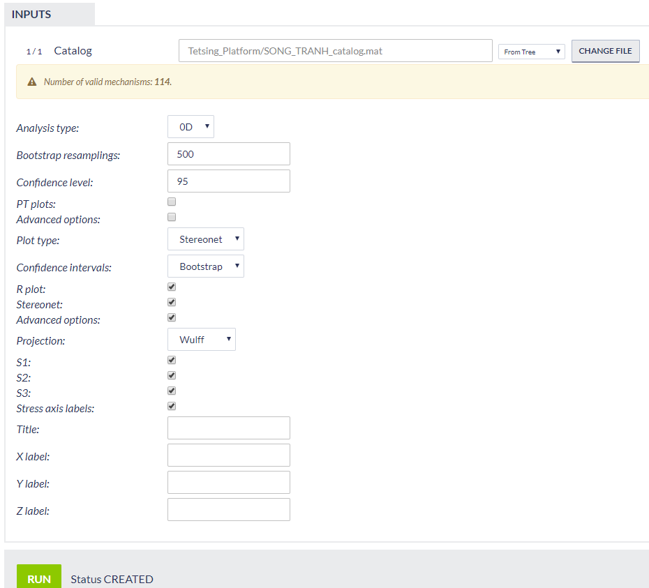
Figure 2. Selection of input parameters and files for the application

Using Seismic Catalog: The seismic catalog has been already selected in the previous step, however, the User may select another dataset from the workspace for stress inversion.

...

Analysis Type: Three options are currently available in the IS-EPOS platform: 0D, 1D and 2D, and can be selected after clicking on the small arrow at the tab. If 1D or 2D options are selected, the user is requested to enter the parameter(s) and window(s) of X, or X and Y dimensions, respectively (Figure 3)

Figure 3. Additional input parameters for the application

Bootstrap Resamplings: Positive integer values are valid in this field, defining the number of Bootstrap Resamplings to be performed. 

...

Advanced Options: A number of advanced options are available after clicking on the small box (Figure 4). See at the MSATSI manual for details (http://www.induced.pl/msatsi)

Figure 4. Additional input parameters for the application

Plot Type: The User may select one of the available options (accordingly to the Analysis Type) after clicking on the small arrow.

...

Advanced Options: A number of advanced options are available after clicking on the small box (Figure 5). See at the MSATSI manual for details (http://www.induced.pl/msatsi)

Figure 5. Additional input parameters for the application

After choosing all the aforementioned parameters the User may click on 'RUN' button to proceed to the calculation process. The results are soon to be available and saved by the system (Figure 6). Those results include schemes, as well as tables with results with option to perform simple plots with those results. These results are shown in the red frame of Figure 7.

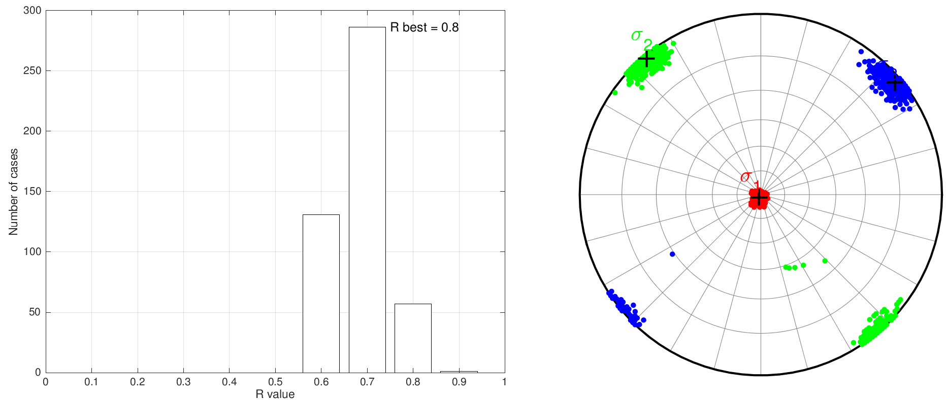
Figure 6. Example of some of the output graphs produced by the application

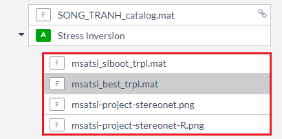
Figure 7. Outputs of the application