Scientific Background
There is no consensus on the a-priori distance-time-size patterns to be selected to relate a given earthquake to a given georesource-reservoir exploitation (e.g . Gupta, 2002, Klose 2013, NRC, 2013). From the one hand, some authors suggest, on observational bases, a 30-50 km distance and 10-20 years times from reservoir to relate an earthquake to a given geo-resource « reservoir » (e.g. for a review Gupta, 2002, Klose 2013) . These a-priori space-time windows question on any of the physics processes that may drive a constant triggering distance to an extended loading source (i.e. not a point source such as a lake surface, or hydrocarbon reservoir). From the other hand, there are evidences that the use of the absolute distance captures earthquake-earthquake triggering patterns (as aftershock-mainshock pair) that hide the key properties of the event interactions (e.g. Bak et al 2002; Parsons and Velasco, 2009, Tahir et al., 2012, Tahir and Grasso, 2015, de Arcangelis et al 2016) . For tectonic earthquake interactions, the size of the triggering zone is mapped by static stress perturbation. This later is estimated to be in the 1-3 L ranges for aftershocks triggering ( Parsons and Velasco 2009; Tahir et al. 2012; Tahir and Grasso, 2015). For the tectonic earthquake analysis (L) is the mainshock fault length as derived from magnitude scale ( e.g. Wells and Coppersmith, 1994) . In order to mimics the earthquake interaction analysis, we choose (L r ) the reservoir length as the equivalent of the mainshock fault length, the characteristic dimension that drives the stress change pattern induced by georesource productions (e.g. Gupta and Rastogi 1976, Bell and Nur, 1978, Roeloffs, 1988; Segall et al. 1994, Deng et al., 2010). This way, in the episodes and applications we uploaded on the platform, we propose to analyse the triggering patterns around geo-resource production using 1-3-10L r normalized distances to the georesource "reservoir", respectively. L r is the characteristic dimension the user defines from the geometry of the georesource production the user work with. Furthermore the rate of aftershocks, whatever the definition, provides information on the proportion of events directly driven by the geo-resource production and the one that are triggered by others earthquake (Helmstetter et al. 2002, Traversa et Grasso 2008, De Arcangelis et al. 2016).
Application objectives:
Anthropogenic seismicity rate and magnitude are analyzed using superposed epochs to extract mean field patterns that are more robust than a single series. This application analyses aftershock sequences in the 1-3L near field distances, L being the Fault length for the earthquake mainshock. Input data are time series from seismicity catalogue. This application is important to quantify the mean field pattern of aftershock production to be compared with regional tectonic patterns. Outputs as aftershock rate over time may be compared to outputs of application "Earthquake interactions - georesource scale".
Tahir, M. , and J-R Grasso. "Faulting style controls for the space–time aftershock patterns." Bulletin of the Seismological Society of America 105.5 (2015): 2480-2497.
De Arcangelis, L, Godano, C, Grasso JR, and E Lippillo, (2016) Statistical physics approach to earthquake occurrence and forecasting, Physic Reports, 628, 1-91
Zaliapin, I., & Ben‐Zion, Y. (2016). Discriminating characteristics of tectonic and human‐induced seismicity. Bulletin of the Seismological Society of America, 106(3), 846-859.
Step by Step
Note:
This service analyses aftershock patterns around mainshock events within normalized distance to the trigger shock targets (L * = L real /(L f(M) ). For example: If mainshocks are selected as M2 events, Lf(M2) is close to 100 m, then the 1-3 L* distances to select aftershocks will correspond to Lreal= 1-3Lf(M2) (i.e. L*= 1 x 100 = 100 m, and 3 x 100 = 300 m, respectively). Accordingly, the user, when using 1-3L* distance to analyze near field triggering, will actually select earthquakes within 100-300 m range. Application inputs are Mm, and (ii) Maft range for triggering and triggered shocks, respectively. To increase the signal-to-noise ratio, we use superposed epoch analysis. It corresponds to the restriction of each time series after a given event to a common t0. Outputs as aftershock rate over time may be compared to outputs of application "Earthquake interactions – georesource scale". We recommend to run the latter mentioned application with the same selection criteria on tectonic seismicity.
After the User adds the Application into his/her personal workspace, the following window appear on the screen (Figure 1):
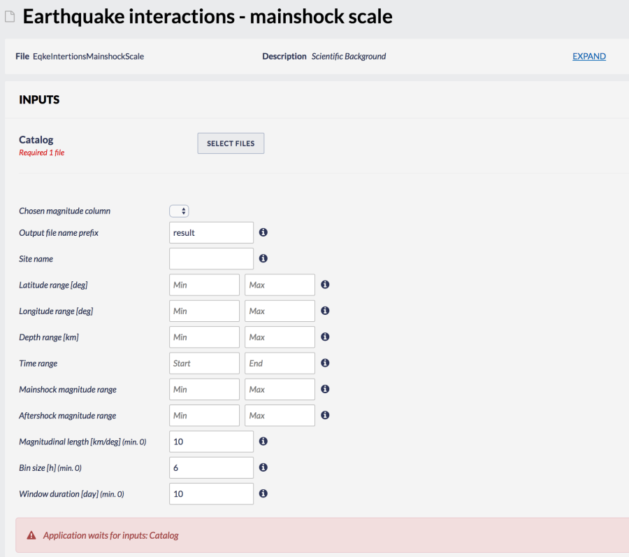
Figure 1. Input window of the "Earthquake Interactions: Mainshock Scale" application.
The User shall click on 'SELECT FILES' button in order to use seismic catalog data among the ones that are already uploaded in his/her personal workspace.
The User is then requested to fill in the fields shown below:
- Chosen Magnitude Column - The user may chose among different magnitude scales (e.g ML, MW), in the Episodes where these scales are available.
- Output file name prefix – File name for the output plot.
- Site name – Name of the site for which the episode is uploaded.
- Latitude range – Range of the latitudes of events to be used for reshuffling analysis.
- Longitude range –Range of the longitude of events to be used for reshuffling analysis.
- Depth range –Range of the depth of events to be used for reshuffled analysis.
- Time range - Range of the time of events to be used for reshuffled analysis. The user can here select a time range to be analysed by clicking boxes.
- Mainshock magnitude range – Range of the magnitude of mainshocks to be used for superposed epoch analysis.
- Aftershock magnitude range – Range of the magnitude of aftershocks to be used for superposed epoch analysis.
- Magnitudinal length – Length deduced from magnitude to count earthquakes in space.
- Bin size – Bin sizes for a given time period.
- Window duration – Number of days before/after that is used for superposed epoch analysis.
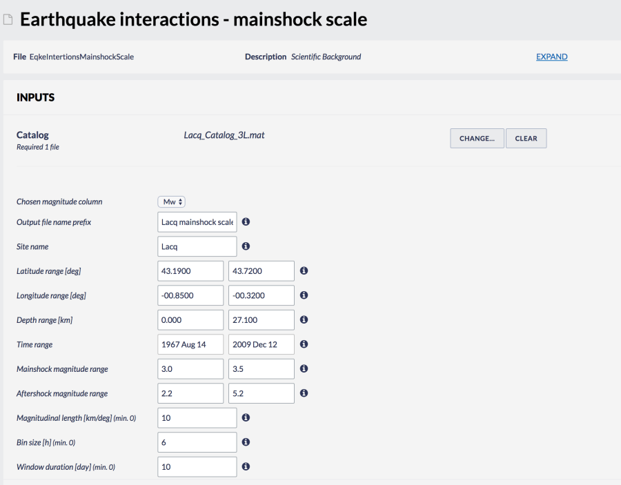
Figure 2. Default values used for the Lacq hydrocarbon field.
After defining the aforementioned parameters, the user shall click on the 'RUN' button and the calculations are performed. The Status changes from 'Submitting' through 'Queued', than 'Running' and finally 'Finished'. The output is created and plotted in the main window just below 'RUN' button. Also the output result appears on the left corner of the platform.
Figure 3 describes the outputs (as time series) of the LACQ field aftershock patterns and they are compared to their Pyrénnées counterpart (same number of events, same magnitude range). It corresponds to seismicity rate in 6h window bins, 10 days before and after N=26 M3-3.5, events. Mean seismicity rate value before and after are in red and blue respectively.
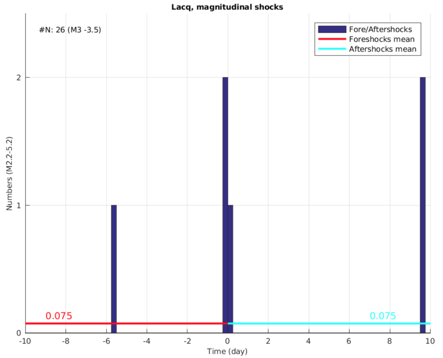
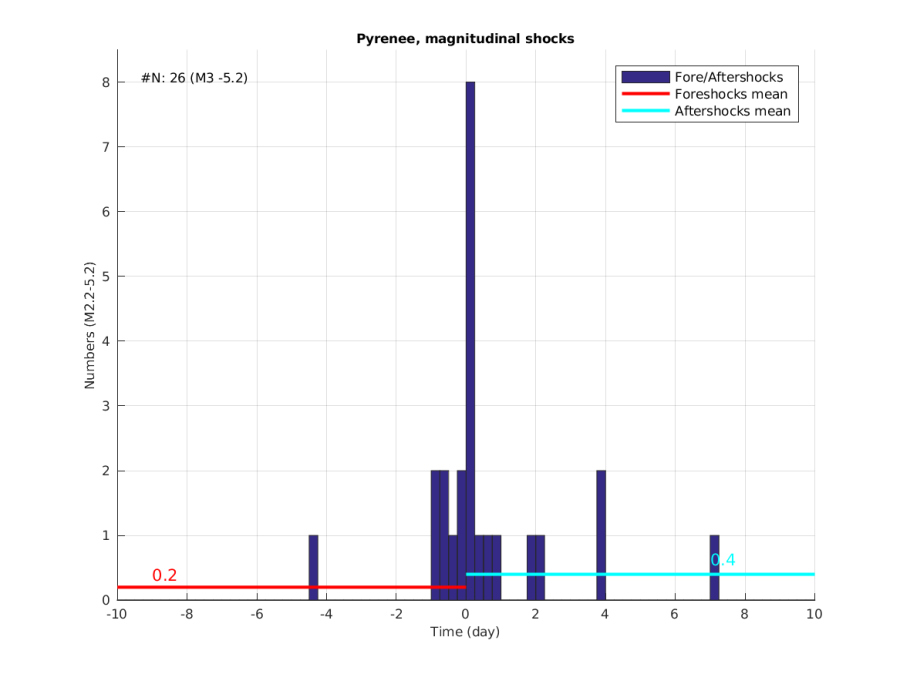
Figure 3. Output histograms "Output file name prefix _gs_length_histograms.png".
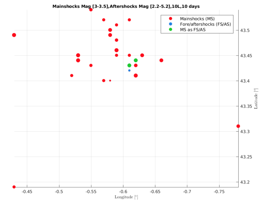
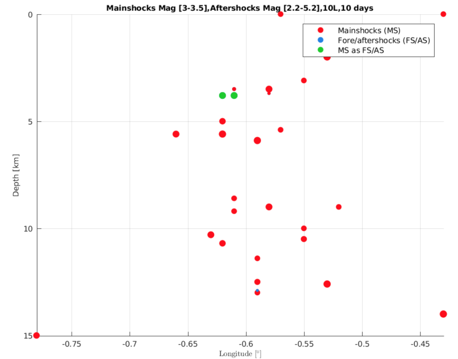
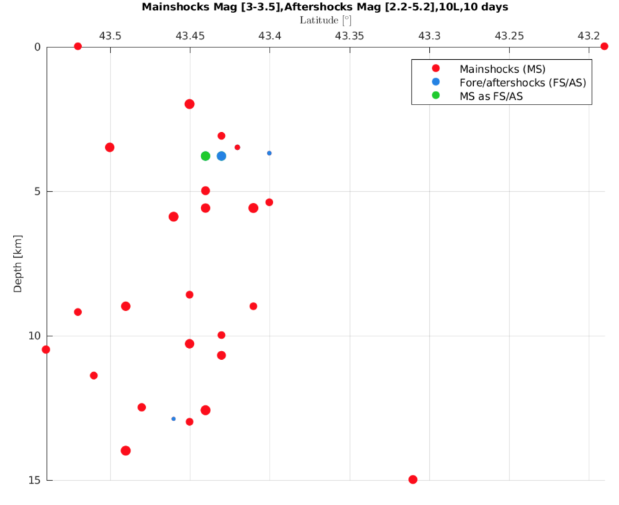
Figure 4. Aftershock analysis (the LACQ field).
Figure 4.: top: map for mainshocks and aftershocks; middle-bottom: cross sections. On the map and cross section, secondary triggering for the target earthquakes are also plotted in Green and Blue.

