Abstract

This application implements a location procedure which allows imaging the distribution of seismic sources in both time and space. Using the predicted arrival times for a set of trial locations and origin times, the code calculates a brightness function by stacking a characteristic function observed at all the stations. The spatial and temporal distribution of sources is then identified by a systematic search throughout the model space and time for the maximum brightness. The main advantage of this procedure is that it exploits waveform information (both arrival times and relative amplitudes) without the need of pre-assembled phase-picking data. The method, therefore, is particularly well-suited for emergent signals and/or for real-time applications. The technique has been largely inspired by the previous works from Kao and Shan (2004), Grigoli et al. (2013, 2014), Langet et al., (2014), to which the reader is referred for a more comprehensive treatment of the methodology.

Method

Consider a seismic source positioned at x₀ acting at time t₀ and radiating a wavefield which is recorded by N receivers located at x. This signal is observed at the i-th recorder at the time t=t₀+T(x₀, x_i), where T is the source-to-receiver travel time.
Now consider a characteristic function CF(t) which results from a transformation of the original signal u(t) aimed at enhancing the energy of the incoming signal, in turn alleviating the waveform distortions due to path and source effects. A brightness function (Kao and Shan, 2004) is then defined as the stack of the time-shifted CFs:

(1)

which also corresponds to the standard beam-forming estimate for the case of arbitrarily-shaped wavefronts. From eq. (1), it is obvious that the B(t) function will attain a maximum when the time shifts x_i applied to the CFs from individual stations correspond to the actual travel times from the source. The procedure begins by parameterizing the volume which is supposed to contain the source(s) with a regular grid of M nodes located at X; travel times T(X, x) are calculated from each of these nodes to all the stations, and stored for subsequent use. Then, an exhaustive grid-search is conducted throughout all the nodes of the mesh: for each tentative source location, the CFs from all the stations are migrated (time-shifted) by the predicted travel times for that node, and then stacked to create a brightness function which is function of time and space (Fig. 1b):

(2)

Whenever the time t and grid node position X correspond respectively to the actual origin time and source location, the CFs will sum in phase thus yelding a maximum for B(t,X).
The procedure is eventually repeated using S-wave travel times, so that a final brightness function is obtained from multiplication of the two individual brightnesses (Grigoli et al., 2013; 2014):

(3)

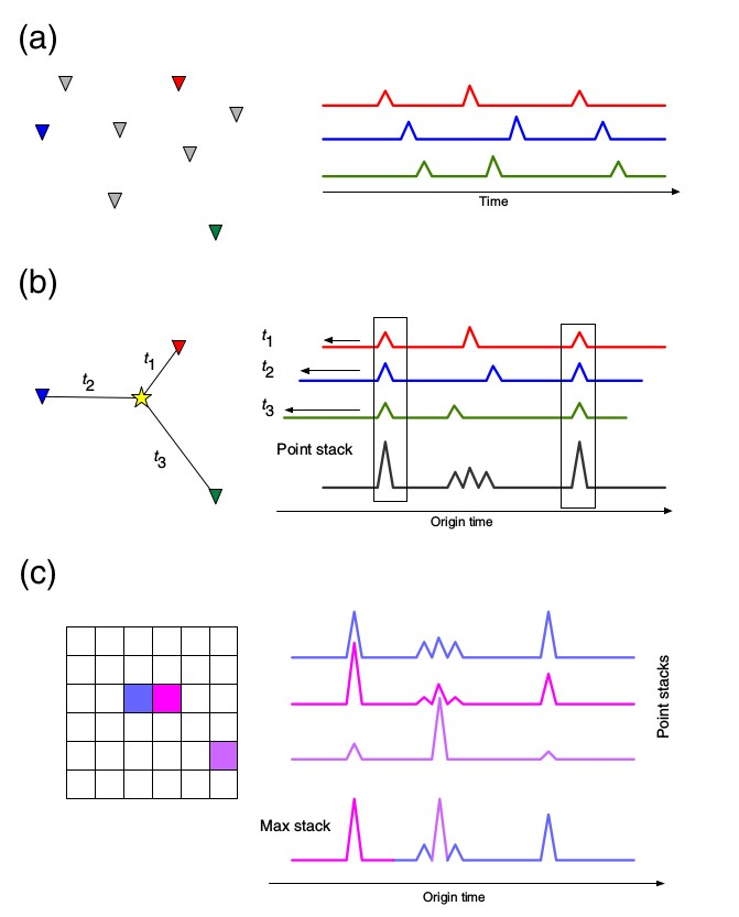
Figure 1. Schematic diagram of the application. (a) Data processing: calculation of an appropriate characteristic function to maximize sensitivity to the presence of seismic events. (b) Migration: the processed waveforms are shifted back in time according to the predicted travel times from a potential hypocentral location, and then stacked. This procedure is repeated for a 3D grid of potential locations, and for both P- and S-waves travel times. (c) At each time step we store the maximum of the point stacks and the location it corresponds to, thereby allowing simple detection and event location.

Implementation details

1. Read seismic data from the N stations. Data are read in SAC format (one file for each station). Station coordinates (lat, lon, elevation) are taken from SAC file's header.
2. Preprocessing. Detrend, demean, taper, band-pass filter within the [f1, f2] frequency band.
3. Decimation. Traces are down-sampled at 0.5 / f2 sampling interval (for instance, if f2 = 10Hz, the new sampling interval dt will be 0.05s, so that the Nyquist frequency corresponds to f2)
4. Alignment. Not necessarily all the traces start and end at the same time. Let's indicate with ts_i and te_i (i = 1, ... ,N) the starting and ending times, respectively, of the different seismograms. The application seeks the smallest starting time (tmin) and the largest ending time (tmax), for building a time vector between of time samples equallyspaced by dt spanning the tmin – tmax interval. Seismograms are then interpolated according to this time vector, so that all the traces start and end at the same time, and are exactly synchronized.
5. Calculation of the STA/LTA function S_i(t). The characteristic function used for the back-projection is given by the short-term-average/long-term-average (STA/LTA) ratio of the energy of the vertical-component signals e(t) = z(t)². For each station, the STA/LTA ratio is calculated using a recursive algorithm described by the following equations (4):
   • sta(i) = ks [c(i)] + (1 − ks) sta(i−1); lta(i) = kl [c(i)] + (1−kl ) lta(i−1), where ns and nl are the number of samples of the short- and long-time windows, respectively, and the index i varies in the range between ns + nl and the last sample of the time series e(t). Following Withers et al. (1999), the decaying constants Ks and Kl are set to 1/ns and 1/nl, respectively.
6. Calculation of predicted Travel Times. In the present implementation, the predicted travel times between the j-th trial source X_j and the i-th recorder located at x_i are calculated assuming a homogeneous medium, and hence: T_ij = || X_j - x_i || / v (5) where v is the user-supplied wave velocity and || indicates the L2-norm.
7. Calculation of the Brightness function B(x{~}j{~},t):

For each trial source j

For each receiver i

Calculate the theoretical travel time T^P_ij for P-wave

Calculate the theoretical travel time T^S_ij for S-wave as T^P_ij /1.73

Calculate the finite time sample corresponding to Tij as tij = 1 + floor(T_ij / dt)

Time-shift of characteristic function: C_i (t + T_ij)

end

Stack C_i, i=1:N to obtain B(x_j, t)

end

For each time sample k

search the location X^max at which B(t_k, X) takes a maximum, and store those time- dependent coordinates of maximum brightness as B'(t_k, X^max).

end

Step by Step

Data Preparation

The User can obtain required SAC files via data conversion as well as by uploading them into his/her workspace from his/her computer.  

Acquiring SEED file of interest: 

• go to 'Data Search' (red field 1, Figure 1), select an episode of interest (red field 2, Figure 1) and select 'Seed Signal' or/and 'Accelerogram Seed Signal' from 'Data Type' (red field 3, Figure 1),

Figure 1. Event waveform selection.

• select an event of interest (here, event #7, Figure 1) by clicking on the 'ADD TO WORKSPACE' button at the right. A prompt window will appear, asking for the directory where to place file in (Figure 2),

Figure 2. Adding waveform to the workspace.

• access your workspace (for more information see My Workspace) and proceed to the directory where you stored your seed data file. Click on it for visualization / checking. It is important that you take note of any bad / noisy channel, as this/these must be ignored in the subsequent location procedure (e.g. station MAR.MR, last signal).

Figure 3. Seed data file visualization.

Data conversion

Seismograms are contained in a seed volume which, for being used in the Waveform-based seismic event location, must be converted to a series of single-channel SAC data files.

WARNING: the format conversion also implies reading of station coordinates from the seed volume (extension .seed), and their writing into the SAC data files header. If the original file is a miniseed volume (extension .mseed) rather than a full seed one, it will not contain stations metadata, and therefore the resulting SAC data files will miss that information and the location procedure will fail.

From Seed Signal view click on the 'ACTIONS' blue button at the top right, choose 'USE IN APPLICATION' tab and than 'SEED to SAC converter'. After successfully running the application the SAC data files will be listed within the 'SeedToSac' directory (Figure 4). See also SEED to SAC converter for more information on the application parameters.

Figure 4. Performing conversion into SAC with the 'SEED to SAC converter' application.

Running the application

Adding the application to workspace:

• from the 'Applications' page (for more information see Applications), choose the 'Waveform-based seismic event location', which will lead you to the description page of the application (Figure 5),

Figure 5. Description of the 'Waveform-based seismic event location' application.

• click on 'Add to Workplace' button at the upper right. A prompt window will appear, asking for the directory where to place the application in, then the User is redirected to his/her workspace and to the application input form (Figure 6). The application form could be later accessed also by choosing the 'WaveformBasedEventLocation' from the tree to the left.

Figure 6. The application input form.

Input Parameters

Vp	P-wave velocity in km/s of homogeneous model. Travel times are calculated for an homogenous, isotropic Earth's model. For source located in the upper 10 km of crust, a value of Vp in between 4 and 6 is generally appropriate. Shear-wave velocities Vs are hard-coded as Vs=Vp/sqrt (3).
Latmin	Minimum latitude of grid within which sources are sought (°, positive N)
Lonmin	Minimum longitude of grid within which sources are sought (°, positive E)
Latmax	Maximum latitude of grid within which sources are sought
Lonmax	Maximum longitude of grid within which sources are sought
zmin	min depth of grid (km below sea level, positive downward)
zmax	max depth of grid (km below sea level, positive downward)
nx	N. of grid nodes along EW direction
ny	N. of grid nodes along NS direction
nz	N. of grid nodes along Z direction

Sources are sought over a volume whose corners at the Earth’s surface are given by [latmin, lonmin] and [latmax, lonmax]. The volume extends from zmin to zmax kilometers beneath the sea level. This volume is then discretised with a mesh of regularly-spaced grid nodes. [nx, ny, nz] indicate the number of grid nodes to use along the longitude, latitude and depth directions, respectively. The higher the number of nodes, the better the possible source(s) will be resolved. At the cost, however, of longer computational times. It is strongly recommended not using number of grid nodes larger than 50-70 along the three directions. To have an idea of the final resolution, just consider an example in which your grid extends along the NS direction by one degree, and that you choose ny=50. Since the length of a latitude degree is on the order of 110 km, your grid nodes along the NS (y) direction will be spaced by about 110/5 = 2.2 km. The same holds for the EW (longitude) extension of the grid, with the difference that the length of a longitude degree depends on the latitude. The grid must encompass the potential source volume, it is necessary an a priori knowledge about the possible location of the signals under examination. If a catalog is available for the selected episode, then you can use the extreme values for latitude and longitude as provided in the informative page of the catalog (Figure 7). If a catalog is not available, a good choice is to use a volume whose horizontal projection includes all the stations which are going to be used in the calculation.

Figure 7. Seismic catalog view.

ws	short window length for sta/lta (s)
wl	long window length for sta/lta (s)

These are the length of the time windows for calculating the short- and long-term averages of the seismograms. There are no obvious choices for setting these values. In general, one wants the STA/LTA ratio to highlight the main phases (P, S), in turn suppressing both the noise preceding the signal of interest and the coda waves following both P and S-wave arrivals. A reasonable choice is to set both wl and ws shorter than the S-P differential time, with a wl / ws ratio on the order of 5. Figure 8 illustrates the effect of different choices of ws and wl.

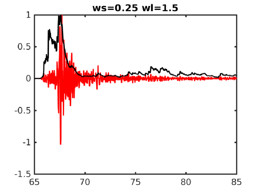
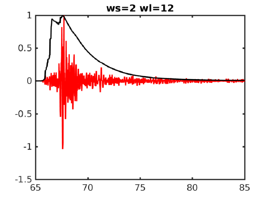
Figure 8. Effects of different window lengths on the calculation of the STA/LTA function. While being noisier, shorter windows preserve details of the main body-wave arrivals.

f1	low corner frequency for filter (Hz)
f2	high corner frequency for filter (Hz)

Minimum and maximum frequency of the band-pass filter. Be careful that f2 must be lower than the Nyquist frequency Fn = 0.5/dt, where dt is the sampling interval of the seismograms. F1 must be higher than the fundamental frequency: f1 > 1/T, where T is the toal time length of the seismogram.

Otype	Output type
A = save the entire B(x,y,z,t) grid R = save only (x,y,z) maxima at each time step

A option: the output is saved as an ASCII file with 5 columns: time, x-location of grid node, ylocation of grid node, z-location of grid node, Brightness as a function of [t, x, y, z]. It may be quite a large file.

R option: the output is saved as an ASCII file with 4 columns: time, x,y,z location of the grid node taking the largest brightness at that particular time.

Results

Graphic files:

• An intermediate plot of the original seismograms and characteristic functions at all the stations:

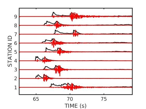
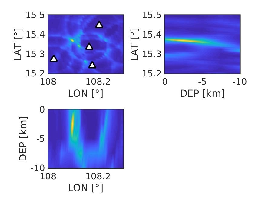
• (x,y), (x,z) and (y,z) brightness sections in correspondence of the time of maximum brightness:

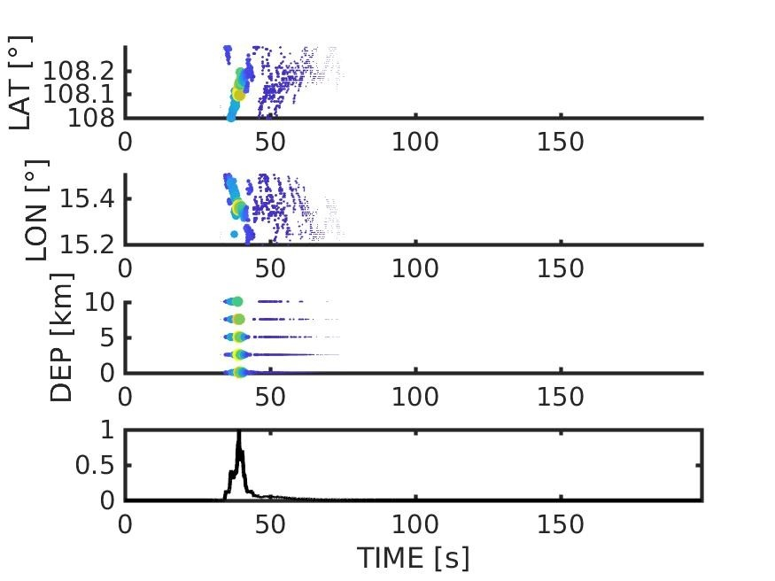
• A final plot of the time-dependent locations of maximum brightness:

Numeric:

• The complete data file containing the space-time dependent brightness B(t,X) or, alternatively, the time-dependent coordinates of maximum brightness B'(t,X^max)

Back to top